
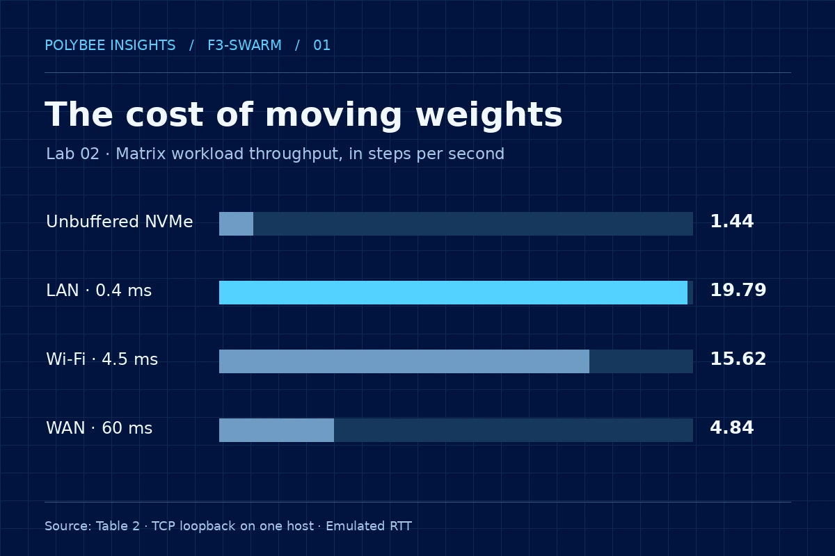
Lab 02 compared repeated matrix reads from NVMe with three processes that kept weights in RAM. In the lowest emulated latency setting, throughput rose from 1.44 to 19.79 steps per second. The result belongs to a controlled matrix workload and helps frame tests for full models.
1. The bottleneck can precede multiplication
Model size tells us how much space its weights occupy, but it does not describe their path during execution. If a layer is absent from memory when its turn arrives, the system has to fetch it. Repeating that transfer on every step turns a loading cost into an operating cost. Even a fast CPU can spend much of its time waiting for data.
Lab 01 recorded 15.788 GiB of physical RAM and 2.789 GiB free at the time of measurement. That snapshot motivates the problem; it is not a fixed memory allowance on any 16 GB computer. Lab 02 created a reproducible per-process cap to compare two ways to fit a 1.50 GiB workload.
2. What the experiment compared
The workload had 24 dense 4,096 × 4,096 float32 layers, with projections, normalization and activations over 32 steps. Each layer occupied 64 MiB. Windows imposed a 600 MiB working-set cap per process. In the SSD arm, one process kept eight layers resident and read the other 16 using unbuffered I/O, preventing the file cache from hiding repeated read costs.
In the resident arm, three workers each kept eight layers and passed 16 KiB activation vectors over TCP on 127.0.0.1. Measured working sets ranged from 529.5 to 546.8 MiB per worker. This works around the per-process cap by using more aggregate RAM: the three working sets summed to about 1.57 GiB. Weight size was not reduced by a comparable amount.
3. What the numbers measure
| Condition | Emulated RTT | Steps/s | Total time | SSD reads |
|---|---|---|---|---|
| Unbuffered NVMe | — | 1.44 | 22.16 s | 33.00 GiB |
| LAN loopback | 0.4 ms | 19.79 | 1.62 s | 0 GiB |
| Wi-Fi loopback | 4.5 ms | 15.62 | 2.05 s | 0 GiB |
| WAN loopback | 60 ms | 4.84 | 6.61 s | 0 GiB |
Telemetry recorded 33.00 GiB of SSD reads and zero in the resident scenarios during the comparison. This volume is measured in the experiment; multiplying nominal streamed layer size by step count yields a simplified calculation, not a substitute for the I/O log. The paper also recorded a maximum numerical difference of 0.0 between the compared outputs.
The useful unit here is steps per second. The preprint labels throughput tok/s, but the measured operation is not text generation by an LLM. Use the reported 13.70× ratio: dividing already rounded table entries gives a slightly different approximation. Numerical parity applies to this computation under these conditions.
4. Transfer size explains the design choice
In the SSD configuration, sixteen 64 MiB layers correspond to a nominal 1,024 MiB of weights read per step. In the three-stage arrangement, there are two transfers of a 16 KiB vector per step: 32 KiB of payload before headers, control and copies. This order-of-magnitude calculation explains why keeping weights at each stage can work. It compares different objects and is not intended to reproduce disk or network counters.
A small payload does not imply a short wait. If the next stage cannot start until its vector arrives, the delay can recur on the critical path on every step. Throughput depends both on bytes per second and on when each message unlocks work. To identify a slowdown, time reading, computation, serialization, sending and waiting for the next stage separately.
5. Separate setup, first step and throughput
Time to the first result and average cost of subsequent steps answer different questions. A short interaction may be dominated by worker setup; a long workload can amortize it. The calculation below uses two reported rates solely to illustrate the point. It does not reproduce telemetry, estimate real loading cost or extrapolate to a production server.
Worked example
When does setup pay off?
Imagine two paths: SSD at 1.44 steps/s and resident weights at 19.79 steps/s, with a hypothetical 2 s setup for resident workers. The calculation is fixed time + steps ÷ throughput. The 2 s setup is illustrative and is not part of Table 2.
In the example, one step takes longer with the 2 s setup; by four steps, higher throughput offsets it. Changing fixed cost or adding concurrency shifts that point. In an applied test, use observed cold and warm startup times, record repetitions and make batch length explicit.
6. First result and sustained pace
Alongside throughput, Table 2 records 715.30 ms to the first result for SSD and 95.33 ms in the emulated LAN setting. Reported subsequent step times are 692.58 ms and 50.54 ms. The emulated Wi-Fi setting reports 59.54 ms to the first result even though its overall throughput is lower than emulated LAN. Comparing only one of these numbers can yield a different conclusion from comparing the entire run.
There is no reason to treat the ordering of these startup timings as a general property of Wi-Fi or LAN: these are loopback observations with injected delay. A stronger protocol controls initial state and reports median and dispersion across repeats. In an interactive application, first output and inter-output intervals deserve separate targets. For batch processing, total time per completed unit may be the primary criterion.
7. What loopback helps isolate
Software injected delays of 0.4, 4.5 and 60 ms. This lets the experiment vary waiting time while keeping the host, workload and process arrangement constant. The decline from 19.79 to 4.84 steps/s shows delay sensitivity in this pipeline. LAN, Wi-Fi and WAN label emulated profiles rather than measurements on physical networks.
On a real network, two paths with the same mean RTT can behave differently. Jitter and retransmissions penalize stages waiting on earlier stages. Bandwidth matters for larger messages; the activation size observed here does not describe every batch and architecture. Hosts with different memory, CPUs and disks can also move the bottleneck. That is why a loopback average cannot serve as a network performance promise.
8. Which comparison answers the engineering decision?
If the question concerns weight movement, holding arithmetic and output constant helps isolate access cost. If it concerns the best deployment for a service, the comparison set changes. Where feasible, include a single resident process, a quantized model that fits in RAM, and a multi-worker pipeline. The gain over SSD does not identify a winner among those alternatives.
Record the total resources consumed by each configuration. Comparing only the largest per-process working set hides aggregate RAM; comparing only throughput ignores first-result time and variability. For real inference, record model settings, quantization, context size, batch and KV cache. Hold inputs constant and verify numerical or quality equivalence as appropriate.
9. Capacity, parallelism and availability
Partitioning a model can solve a capacity problem even when it does not shorten one request. A pipeline divides weight residency; for one request, its dependencies remain sequential. Serving multiple requests may change stage utilization, but adds queues and requires memory and concurrency limits. Record service throughput and per-request latency as separate metrics.
A single-host test also does not reveal what happens when a worker becomes unavailable. In a physical implementation, test failures, reconnection and a local execution fallback under the same budget and equivalent inputs. A speed gain during healthy execution may cease to pay off when transfers fail often or when the cost of keeping hosts available outweighs the benefit.
10. A protocol for moving beyond the lab
First reproduce the single-host control with the recorded data and settings. Then place workers on two or more hosts, preserve the measured operation and change one condition at a time. Observe SSD reads, total resident memory, bytes transferred and per-stage timing. Report cold and warm runs and latency distributions, including p95, rather than only the best run.
Finally, run a complete model with attention, embeddings and cache, measuring tokens and quality against the same reference configuration. This tests a new hypothesis. F3-Swarm’s model cascade was evaluated locally in another track; the matrix benchmark did not integrate it with a multi-host network. This track’s contribution is to show under which measured conditions movement costs change the architecture choice.
Questions to keep exploring
Does 13.70× apply to text generation?
Text generation was not measured. The figure applies to matrix workload throughput versus unbuffered SSD at 0.4 ms emulated RTT.
Does the technique save total RAM?
The experiment redistributes weights across processes. It does not demonstrate lower aggregate RAM.
Can SSD still be the best option?
Yes, depending on memory, setup, workload reuse and latency targets. Measure the configuration of interest.
What remains to show a gain on a real network?
Run on separate hosts and measure networking, variability, total memory and quality with a full model and comparable baselines.
Sources and references
The sources below document the experiments. Editorial examples are identified separately from measurements.
- Polybee AI ResearchF3-Swarm v1.5.2 · technical preprint
Manuscript, experimental design and limitations.
- ZenodoF3-Swarm v1.5.2 · DOI 10.5281/zenodo.24095260
Persistent research record.
- Polybee AI Researchlab02_physical_results.json
Telemetry used in Table 2.
- Polybee AI Researchf3_swarm_lab02_physical_test.py
Implementation of the memory comparison.