
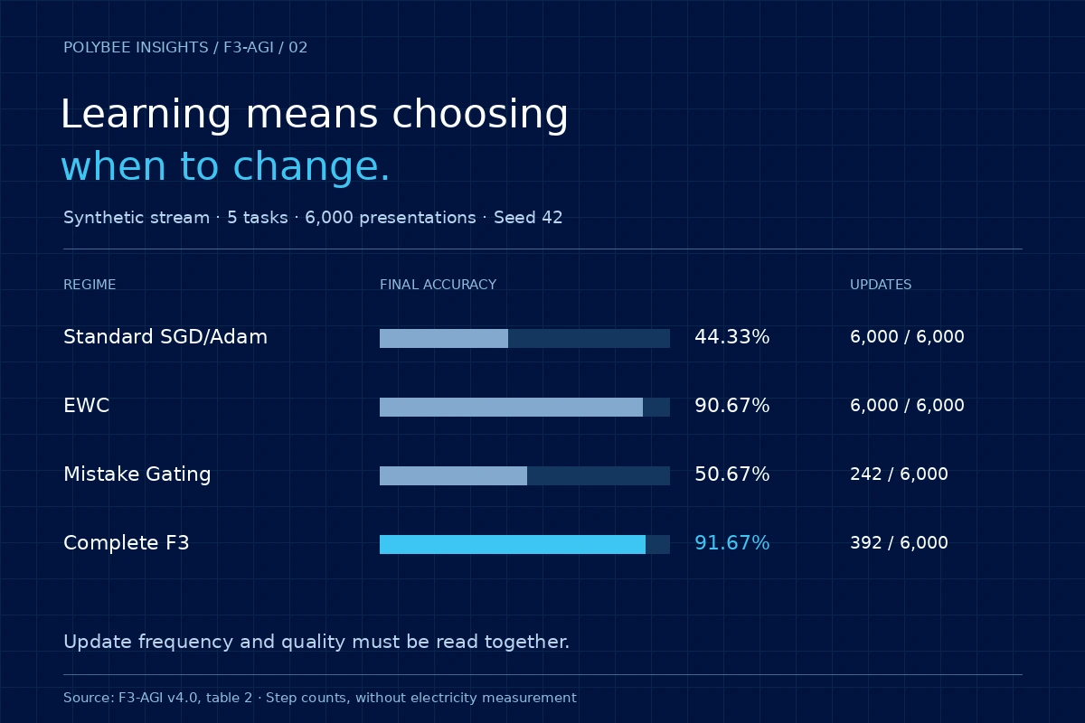
In the F3-AGI v4.0 synthetic experiment, the complete regime retained 91.67% final average accuracy while executing 392 updates across 6,000 presentations. The result opens a discussion of selective learning: skipping more updates alone did not guarantee better memory. Evaluating efficiency requires examining retained quality, the frequency and magnitude of changes, and the actual cost of running the whole system.
1. Learning something new can displace what already worked
Imagine a classifier that first learns to distinguish two types of signal. It then receives a new pair of categories and adjusts the same parameters. If the shared representation changes too much, decisions that worked in the first stage may deteriorate. The system can finish highly competent on the recent task and unreliable on earlier ones.
This makes final-task accuracy an insufficient description. In continual learning, we also need to know what remains accessible after the entire sequence. The choice involves plasticity, to incorporate new information, and stability, to preserve earlier skills. Simply freezing every parameter would preserve some of the past, but could prevent useful learning.
Elastic Weight Consolidation, or EWC, proposes protecting parameters important to earlier tasks through a penalty that makes moving them harder. Kirkpatrick and colleagues provide the context for this retention strategy. Their work also reminds us that preserving memory requires an explicit mechanism and comparison with suitable alternatives. [1]
The F3-AGI continual-learning study investigates another dimension of this trade-off: when is an update worth executing? The engineering hypothesis is that adapting the frequency and direction of changes can preserve performance with fewer interventions in the weights. To examine it, we first need to delimit the tested setting and what was actually counted.
2. A controlled experiment with explicit boundaries
The evaluation uses five sequential tasks, each with two classes, in a synthetic 64-dimensional feature space. A network with layers 64 → 256 → 128 → 10 receives 120 training examples per task over ten epochs, totaling 6,000 presentations. Testing uses 60 examples per task. The published configuration uses seed 42. [2] [3]
Here, “zero replay” means that training on new tasks does not retrieve a buffer of examples from previous tasks. Examples are repeated during the current task’s ten epochs. This distinction matters: the evidence does not describe a stream in which each sample is seen only once, or a system without any internal memory. The algorithm maintains statistics and consolidation information.
Inputs are already synthetic vectors constructed from prototypes. The experiment does not train directly on raw ARC grids, natural images or language. This isolates inter-class interference and update mechanisms at low cost. It also limits immediate transfer of the conclusions to tasks requiring the perceptual representation itself to be learned.
The record contains four regimes: standard updating, EWC, mistake gating alone and complete F3-Metabolic-Optim. The report calls the first condition “SGD/Adam”; the implementation of that path applies a direct update proportional to the gradient. We therefore treat the numbers as a comparison of the published implementations, without extending them to every optimizer bearing those names. [4]
This care keeps a controlled test from becoming a universal claim. The setting is useful because it investigates a specific hypothesis. Its evidence becomes stronger when other conditions preserve the conclusion, particularly changes to task order, noise, network size and example distribution.
3. Three decisions: whether to update, in which direction and by how much
The first decision gates entry into learning. In the implementation, the need for an update depends on the error associated with the correct class and a memory of problematic examples. If an example already satisfies the criterion and no longer remains in that memory, the weight-changing step can be skipped. A forward pass still occurred to produce the prediction and evaluate the gating condition.
The second decision concerns the direction of change. The complete regime uses parameter-importance statistics, preconditioning and attraction toward consolidated weights. The intention is to reduce interference in directions associated with prior knowledge. Skipping steps does not produce that effect automatically: an executed update can still displace parameters useful to other tasks.
The third decision modulates magnitude. An internal tensor called M influences the update through a control function and changes during execution. “Metabolic” terminology describes the algorithm’s inspiration and organization. It does not establish equivalence with cellular processes or provide a conversion into hardware energy consumption. [4]
When to change
Error and its memory guide the execution or skipping of an update step.
What to protect
Historical importance and consolidated weights constrain parameter displacement.
How much to change
An internal algorithmic state adjusts the magnitude of executed changes.
Separating these decisions helps interpret results and plan ablations. Comparing four regimes does not, by itself, identify the causal contribution of every term in the complete regime. Doing so would require varying components while maintaining the other controls: initialization, stream, tuning budget and multiple repetitions.
Deciding to do nothing also has a cost. Evaluating error, consulting memory and maintaining statistics require work. A count of skipped steps reveals an important part of execution; total accounting must include the operations that made that selection possible.
4. The regime that skips the most updates does not retain the most
The figures below are the author’s published results, with no new execution for this essay. Accuracy is the mean across five tasks after training on the fifth. The forgetting column follows the report’s percentage terminology; in the code, it is calculated as the mean drop, in accuracy percentage points, from the best recorded value to the final value on the four earlier tasks. [3] [4]
| Published regime | Final accuracy ↑ | Forgetting ↓ | Executed steps | Skipped steps | M1 ↓ |
|---|---|---|---|---|---|
| Standard SGD/Adam | 44.33% | 69.58 | 6,000/6,000 | 0.00% | 3,433.87 |
| EWC | 90.67% | 11.25 | 6,000/6,000 | 0.00% | 7,986.85 |
| Mistake Gating alone | 50.67% | 61.25 | 242/6,000 | 95.97% | 3,040.31 |
| F3-Metabolic-Optim | 91.67% | 9.17 | 392/6,000 | 93.47% | 2,736.81 |
Gating alone executes 150 fewer steps than complete F3. Even so, its final average accuracy is 50.67%, with greater forgetting. This shows why maximizing the percentage of skipped steps can select an unsuitable regime when preserving competence throughout a sequence matters.
The EWC comparison answers another question. In this run, F3 reaches similar final accuracy with fewer steps and a lower cumulative magnitude of change. However, the one-percentage-point accuracy difference has no uncertainty interval estimated across multiple seeds. It should remain an observed difference in this configuration.
Per-task results add information hidden by the mean. At the end, the record shows 75% on the first task for F3 and 65% for EWC; the other tasks vary in both directions. A future evaluation should preserve the performance matrix throughout the sequence, making it possible to locate when a skill was acquired, forgotten or recovered.
5. Updates, M1, time and energy answer different questions
In the published counter, a “synaptic update” is a step in which the network’s parameters change. The number 392 does not count 392 individual connections: each step can update many weights. The measure reports intervention frequency relative to the 6,000 presentations.
M1 adds the magnitude of those interventions: M1 = Σₜ Σᵢ |Δwₜ,ᵢ|. Two regimes can execute the same number of steps while moving their parameters at very different scales. F3 records M1 of 2,736.81, compared with EWC’s 7,986.85, approximately 65.7% lower on this indicator. This calculation depends on parameterization, weight scale and which changes are counted. [2]
Runtime includes other components: forward passes, gradient calculation, consolidation, memory access and implementation overhead. The published artifacts even contain different timings: manuscript table 2 reports approximately 1.06 s for F3 and 2.32 s for EWC; the release JSON records 1.554 s and 5.073 s. These are distinct records that should not be combined into a single speedup estimate. [2] [3]
Electrical energy requires documented physical measurement or estimation, with power integrated over time. Emissions additionally involve the carbon intensity of electricity and the chosen scope. Strubell and colleagues’ discussion of training costs helps motivate this attention, without supplying a ready conversion for our experiment. [5]
Virtual ATP is a program control state. Interpreting it as battery charge, joules or real molecules would invent a unit the study did not measure. Biological analogy can guide mechanisms; computational validation and biological validation still require their own experiments.
6. A simple calculation shows the role of the cost that remains
We can construct an accounting illustration without estimating F3’s consumption. Suppose a dense process costs 100 normalized units. Some fraction belongs to updates that can be avoided; the remainder persists, including operations required for every presentation. Assume, only for this model, a uniform cost per step and no additional overhead from the selective mechanism.
If the avoidable share is 20 units and we execute 392/6,000 updates, the illustrative cost becomes 80 + 20 × (392/6,000) ≈ 81.31. The total reduction is approximately 18.69%, even though 93.47% of update steps were skipped. The difference comes from the accounting scope: much of the work remains.
Illustrative accounting model
How much of the cost can be avoided?
Reference: 100 units. Fraction of updates executed: 392/6,000.
normalized units
relative to the 100 units
The remaining share is held constant. The model ignores selection overhead, differences between updates and hardware effects.
Mathematical demonstration, without energy measurement or F3 execution. The control changes an assumed cost share, rather than an experimental observation.
When the avoidable share approaches zero, skipping updates has little effect on the total. When it dominates the process, skipped steps can matter more. The model helps identify the missing measurement: how much does each part actually cost under the conditions of use?
In a real implementation, cost per update may also vary. Small operations may use hardware poorly; memory access may dominate runtime; complex selection may consume part of the expected saving. These possibilities require measurement. The demonstration offers a way to design that measurement without anticipating its outcome.
7. Measuring efficiency from end to end
A future protocol can treat efficiency as the relation between delivered quality and resources consumed. Green AI advocates including efficiency among evaluation criteria and reporting computational costs. For our next round, this translates into concrete experimental choices proposed here by the author. [6]
- Define the functional unit.
For example: complete the same task sequence while retaining a minimum final accuracy. Comparing cost without controlling quality can reward a system that simply learns less.
- Fix the execution scope.
Include predictions, gating, gradients, consolidation and evaluation when they belong to the declared use. Report development cost separately from the cost of a frozen execution.
- Record physical conditions.
Identify the processor, memory, system, libraries, thread count, warm-up and concurrent processes. State whether the measurement covers a process, a component or the entire machine.
- Repeat duration and energy measurements.
Document the instrument or estimator, sampling frequency and handling of idle consumption. Publish raw values and dispersion, using the same convention for every regime.
- Keep the algorithmic metrics.
Step counts, M1 and memory help explain behavior. Relating these indicators to physical measurements allows us to test when they work as useful proxies and when they stop doing so.
This protocol also needs equivalence criteria. If a regime reaches the required quality with less training, comparing only a fixed duration may hide its advantage. If another depends on extensive hyperparameter tuning, ignoring that process hides part of the cost of obtaining it. Both views should be reported with explicit boundaries.
8. Where selection can fail is part of the hypothesis
An example that appears solved today may require learning again after a distribution shift. Overly conservative gating risks recognizing the need to adapt too late. Overly sensitive gating may reactivate frequent changes and lose the expected saving. Varying the strength and speed of the shift directly tests that trade-off.
Rare information also matters. An infrequent class may contribute little to the mean while being decisive for an application. We propose tracking per-class performance, update activation frequency and time since the last change, to investigate whether selectivity allocates resources usefully or reinforces stream imbalances.
Task order deserves the same care. A regime may benefit from a sequence whose representations complement one another and struggle when similar tasks require incompatible decisions. Repetitions with permutations, new seeds and different noise levels should include individual results, allowing variation to be observed beyond a final mean.
The comparison between the complete regime and gating alone already provides a testable question: how much retention depends on weight consolidation, how much on preconditioning and how much on internal modulation? A factorial ablation with a comparable parameter-selection budget would help separate these contributions. It should also account for stored statistics and consolidation time.
Finally, moving from synthetic vectors to more complex inputs may shift the bottleneck toward representation. If the dominant cost lies before the skipped step, the same skipping rate has a different operational significance. This is a reason to publish the execution profile alongside the learning result.
9. A refutable agenda for selective learning
The current result supports a bounded investigation: in this synthetic configuration, combining update selection and retention mechanisms achieved high final average accuracy with few weight-changing steps. The regime that skipped the most steps in isolation did not best preserve the tasks. This is a useful starting point for harder experiments.
A next contribution would demonstrate that the quality–cost relationship persists across new seeds, orders and distributions, with broader comparisons and physical measurements. Another would identify conditions in which the mechanism fails: recognizing them helps refine the hypothesis and choose where the approach is useful.
For the community, we propose reporting efficiency with a denominator and a quality commitment. How many steps were avoided? What work remained? What was retained? What did the entire system cost? These questions allow mechanisms to be compared without automatically turning a promising algorithmic idea into an environmental claim.
The institutional research page provides the preprint, code and software DOI. Reproductions recording hardware, version, configuration and complete results can turn this initial experiment into cumulative evidence. In the series’ third article, the same attention to cost appears at another scale: the actions of an agent that must discover how an environment works.
Questions to keep exploring
Does skipping 93.47% of updates mean using 93.47% less electricity?
No. The percentage divides skipped update steps by the 6,000 presentations. The system still executes predictions and control mechanisms. Estimating electricity savings requires physical measurements and a defined comparison scope.
Does the experiment demonstrate continual learning on ARC grids?
It uses 64-dimensional synthetic features, five tasks and a small network. The static ARC grid study is a separate experiment in the preprint. Results must remain associated with their respective protocols.
What does the forgetting metric mean?
In the published implementation, it is the mean accuracy drop, in percentage points, from the best recorded value to the final value on the four earlier tasks. The report calls it forgetting_ratio_pct. It does not represent a percentage of forgotten weights.
Were new measurements performed for this article?
No. The essay analyzes the preprint and artifacts from release v4.0.0. The interactive control is an illustrative accounting model; the proposed measurement and robustness checks are a future agenda.
Sources and references
Literature and documentation consulted on October 30, 2026. F3-AGI results are those reported in the preprint and the author’s records; no new benchmark runs were performed for this essay. Teaching examples, interpretations and proposed evaluations are identified in the text.
- James Kirkpatrick and colleaguesOvercoming catastrophic forgetting in neural networks
Primary work on EWC. Context for protecting important parameters during sequential learning.
- Henrique Oliveira / Polybee AI ResearchF3-AGI v4.0 — preprint
Manuscript dated October 29, 2026, without peer review. Sections 3.4 and 5.1, table 2. Its published timings differ from those in the release JSON.
- Polybee AI Researchf3_metabolic_optim_results.json — release v4.0.0
Configuration, seed 42, metrics for all four regimes and recorded execution times. Results produced by the author.
- Polybee AI Researchf3_metabolic_optim.py — v4.0.0 implementation
Code for the synthetic stream, gating, parameter updates, consolidation and metrics. Consulted to establish the meaning of the counters.
- Emma Strubell, Ananya Ganesh and Andrew McCallumEnergy and Policy Considerations for Deep Learning in NLP
2019 work on financial and environmental costs of NLP training. General context, without transferring estimates to F3.
- Roy Schwartz, Jesse Dodge, Noah A. Smith and Oren EtzioniGreen AI
2019 work advocating evaluation and reporting of efficiency alongside performance. The protocol suggested in this essay is an original editorial proposal.
- Polybee AI ResearchF3-AGI v4.0.0 — software DOI
Software artifact identifier, according to the release reference. It does not identify arXiv publication of the manuscript, which is awaiting endorsement.